10.7 preview feature JSON Histograms

MariaDB has had support for histograms as part of Engine Independent Table Statistics since 10.0. As part of Google Summer of Code (MDEV-21130), Michael Okoko, together with his mentor Sergey Petrunia, have implemented a new format (using JSON) for histograms that significantly improves the accuracy and flexibility of histograms. For those just interested in the feature details, you can skip to the “New format”, however if one is unfamiliar with the purpose of histograms, read on.

Why statistics are needed

Histograms are important for queries where the WHERE clause uses columns that are not indexed. When columns are not indexed, the optimizer has limited information available.

To make this more apparent let’s imagine the following situation: we have two tables customers and orders. Let’s say we want to find out which customers younger than 30 have orders greater than 10000€. We assume each table has a primary key and also the foreign key has an index. The query given to the optimizer is:

SELECT c.name as 'Customer Name', c.age as 'Customer Age'
       o.date as 'Order Date', o.total_sum as 'Order Total Invoice' 
FROM customers c JOIN orders o ON customers.id = orders.customer_id
WHERE orders.total_sum >= 10000 and c.age < 30

Depending on the type of store and what kind of goods it’s selling, we could have many orders matching this query (for example a car dealership) or none at all (for example a thrift store). It’s all down to the data distribution. This means that the query optimizer needs to make a choice: does it start the scan from customers and look up each order, or does it start the scan from orders and looks up the customer data?

Without column statistics, the optimizer will assume that all conditions have a selectivity of 100%, which means that all rows will pass both conditions. This means that the only viable option is to start with the smaller table, which is customers. But this is not always the right choice. It could be that there is only a very small fraction of orders that match, in which case it makes little sense to join all the customer data only to discard it afterwards. That’s why the query optimizer needs column statistics.

The old format

In 10.0, MariaDB introduced support for collecting statistics via ANALYZE TABLE ... PERSISTENT FOR ALL. The format was a binary representation of a height-balanced (or equi-height) histograms that can not be bigger than 255 bytes in size. Additionally, the histogram precision could be set to single or double precision (one or two bytes per bucket).

There are multiple problems with this format:

1. The bucket boundaries are hard to accurately define (especially for text-based data)
2. The representation is not very flexible. It can not cover other types of histograms, such as most-common-values.
3. Examining histogram data is not user friendly (even with the DECODE_HISTOGRAM function).
4. Skewed data (such as a very common value among lots of single occurrences) can make the histogram useless. This is the case with names for example.
5. The single precision type has limited precision (of only 255 levels), making it prone to rounding errors for most distributions and even the double precision still has the limitation of 255 * 255 levels.

To illustrate these problems, here are two distributions that were collected using MariaDB’s analyze table, with double precision histograms. First, a good use case. A normal (Gaussian) distribution of values.

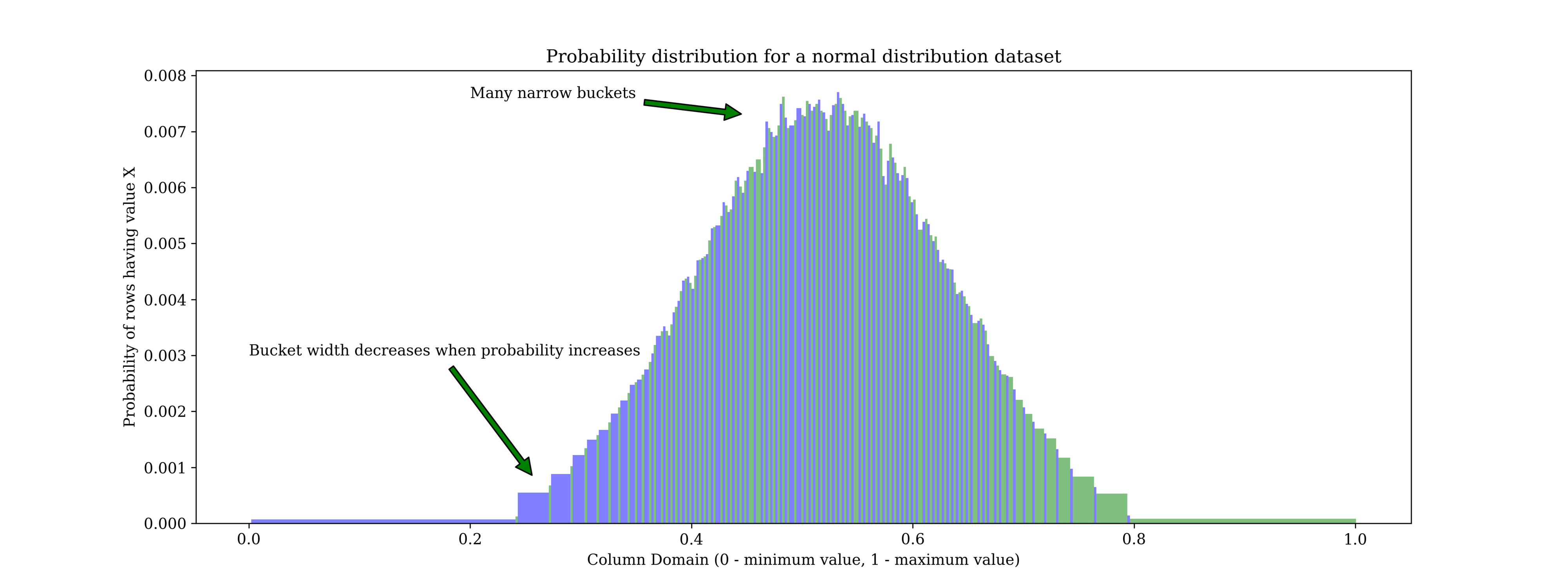
Here we can see the advantage of equal-height histograms. Where the data distribution is low, there are few buckets to cover the range. (For example from 0 to 0.2, there is only one bucket). As the data distribution increases between 0.4 and 0.6 data range, the buckets get narrower, giving greater precision for the “interesting” areas.

Now let’s look at the poorly performing use case. A histogram showing names probability distribution.

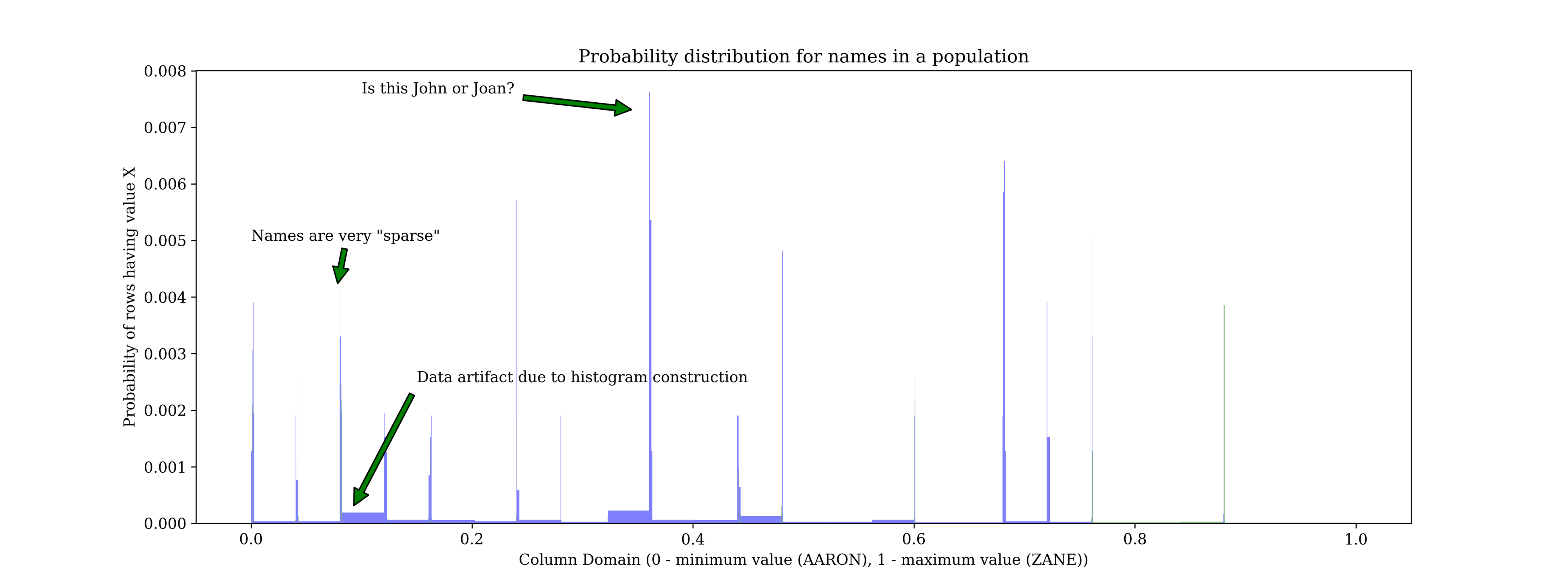
Here we can see the sparse nature of names. Our domain starts with AARON and ends with ZANE, but it has plenty of potentially invalid names in between, like AARPN or ZAME or ZAAZBBB. The representation can not account for this. We even end up with a few artifacts where we have a uniform distribution between peaks.

The new format

Given the limitations of the old format, we have decided to introduce a more flexible representation using JSON. Let’s have a look at the changes:

For one, the mysql.column_stats table has had its histogram column type changed to blob, so it can cover both the old format and the new one. The type column now accepts JSON_HB. The system variable histogram_type system variable accepts this new type. When the type is set to JSON_HB, the variable histogram_size specifies the number of buckets the histogram will contain.

The histogram itself now looks like this (3 buckets for this example):

{
  "histogram_hb_v2": [
    {
      "start": "Berlin",
      "size": 0.333333333,
      "ndv": 1
    },
    {
      "start": "Paris",
      "size": 0.333333333,
      "ndv": 1
    },
    {
      "start": "Rome",
      "end": "Rome",
      "size": 0.333333333,
      "ndv": 1
    }
  ]
}

The key identifies the version of the histogram. This will change in future MariaDB versions. For this particular version, the data is an array of buckets. Each bucket specifies the start of the histogram bucket. This is the first value in the data range that that fits within the bucket. The end value is specified only for the last bucket, as for the previous buckets the optimizer uses the following bucket’s start as the current bucket’s end.

Then we have the size, which signifies the fraction of rows (out of all the rows in the table) that fit within this bucket. For most datasets, the size will tend to be the same (or very close) for all buckets, but if there is a very common value, that one will get its own bucket and could hold a much bigger fraction out of the total table rows. For these buckets you will notice that ndv (which is the total number of distinct values that fit within the bucket) is set to 1.

If we compare performance for our names example:

With old representation, look at filtered column to see the percentage of rows that the histogram predicts and r_filtered to see what the query actually returned:

MariaDB [statistics]> analyze select * from t2 where names = 'John';
+...+-------------+-------+...+--------+-----------+----------+------------+
|...| select_type | table |...| rows   | r_rows    | filtered | r_filtered |
+...+-------------+-------+...+--------+-----------+----------+------------+
|...| SIMPLE      | t2    |...| 100000 | 100000.00 |     5.47 |       3.63 |
+...+-------------+-------+...+--------+-----------+----------+------------+
1 row in set (1.141 sec)

With JSON representation:

MariaDB [statistics]> analyze select * from t2 where names = 'John';
+...+-------------+-------+...+--------+-----------+----------+------------+
|...| select_type | table |...| rows   | r_rows    | filtered | r_filtered |
+...+-------------+-------+...+--------+-----------+----------+------------+
|...| SIMPLE      | t2    |...| 100000 | 100000.00 |     3.63 |       3.63 |
+...+-------------+-------+...+--------+-----------+----------+------------+

So for John, the old histogram doesn’t look that bad. It is not exact, but it is not that far off. However, let’s try Joan, a name very close to John.

With old representation:

MariaDB [statistics]> analyze select * from t2 where names = 'Joan';
+...+-------------+-------+...+--------+-----------+----------+------------+
|...| select_type | table |...| rows   | r_rows    | filtered | r_filtered |
+...+-------------+-------+...+--------+-----------+----------+------------+
|...| SIMPLE      | t2    |...| 100000 | 100000.00 |     5.47 |       0.01 |
+...+-------------+-------+...+--------+-----------+----------+------------+

With JSON representation:

MariaDB [statistics]> analyze select * from t2 where names = 'Joan';
+...+-------------+-------+...+--------+-----------+----------+------------+
|...| select_type | table |...| rows   | r_rows    | filtered | r_filtered |
+...+-------------+-------+...+--------+-----------+----------+------------+
|...| SIMPLE      | t2    |...| 100000 | 100000.00 |     0.08 |       0.01 |
+...+-------------+-------+...+--------+-----------+----------+------------+
1 row in set (1.141 sec)

And here we see the difference! For the old format, Joan and John fall in the same bucket and thus produce the same estimate, where one is wildly off. (5% instead of 0.01%). The new format reduces this error down to 0.08%, 2 orders of magnitude better!

We believe this feature will help improve the optimizer’s overall performance, for many use cases. We are especially looking for feedback now, while the iron is hot and we can work out any limitations we may have missed. Let us know how the optimizer fares with the new histograms with your data and queries!

How to try the 10.7 JSON histograms yourself?

Tarball

Go to tarball downloads.

Container

To test this preview release with as little effort as possible, you can run the container called quay.io/mariadb-foundation/mariadb-devel:10.7-mdev-26519-improved-json-histograms with the same interface as the Docker Library mariadb image.

Feedback welcome

If you come across any problems in this feature preview, with the design, or edge cases that don’t work as expected, please let us know with a JIRA bug/feature request on the MDEV project. You are welcome to chat about it on Zulip.

See also the Knowledge Base page for further details.